This new series of articles focuses on working with LLMs to scale your SEO tasks. We hope to help you integrate AI into SEO so you can level up your skills.
We hope you enjoyed the previous article and understand what vectors, vector distance, and text embeddings are.
Following this, it’s time to flex your “AI knowledge muscles” by learning how to use text embeddings to find keyword cannibalization.
We will start with OpenAI’s text embeddings and compare them.
| Model | Dimensionality | Pricing | Notes |
|---|---|---|---|
| text-embedding-ada-002 | 1536 | $0.10 per 1M tokens | Great for most use cases. |
| text-embedding-3-small | 1536 | $0.002 per 1M tokens | Faster and cheaper but less accurate |
| text-embedding-3-large | 3072 | $0.13 per 1M tokens | More accurate for complex long text-related tasks, slower |
(*tokens can be considered as words words.)
But before we start, you need to install Python and Jupyter on your computer.
Jupyter is a web-based tool for professionals and researchers. It allows you to perform complex data analysis and machine learning model development using any programming language.
[embedded content]
Don’t worry – it’s really easy and takes little time to finish the installations. And remember, ChatGPT is your friend when it comes to programming.
In a nutshell:
- Download and install Python.
- Open your Windows command line or terminal on Mac.
- Type this commands
pip install jupyterlabandpip install notebook - Run Jupiter by this command:
jupyter lab
We will use Jupyter to experiment with text embeddings; you’ll see how fun it is to work with!
But before we start, you must sign up for OpenAI’s API and set up billing by filling your balance.
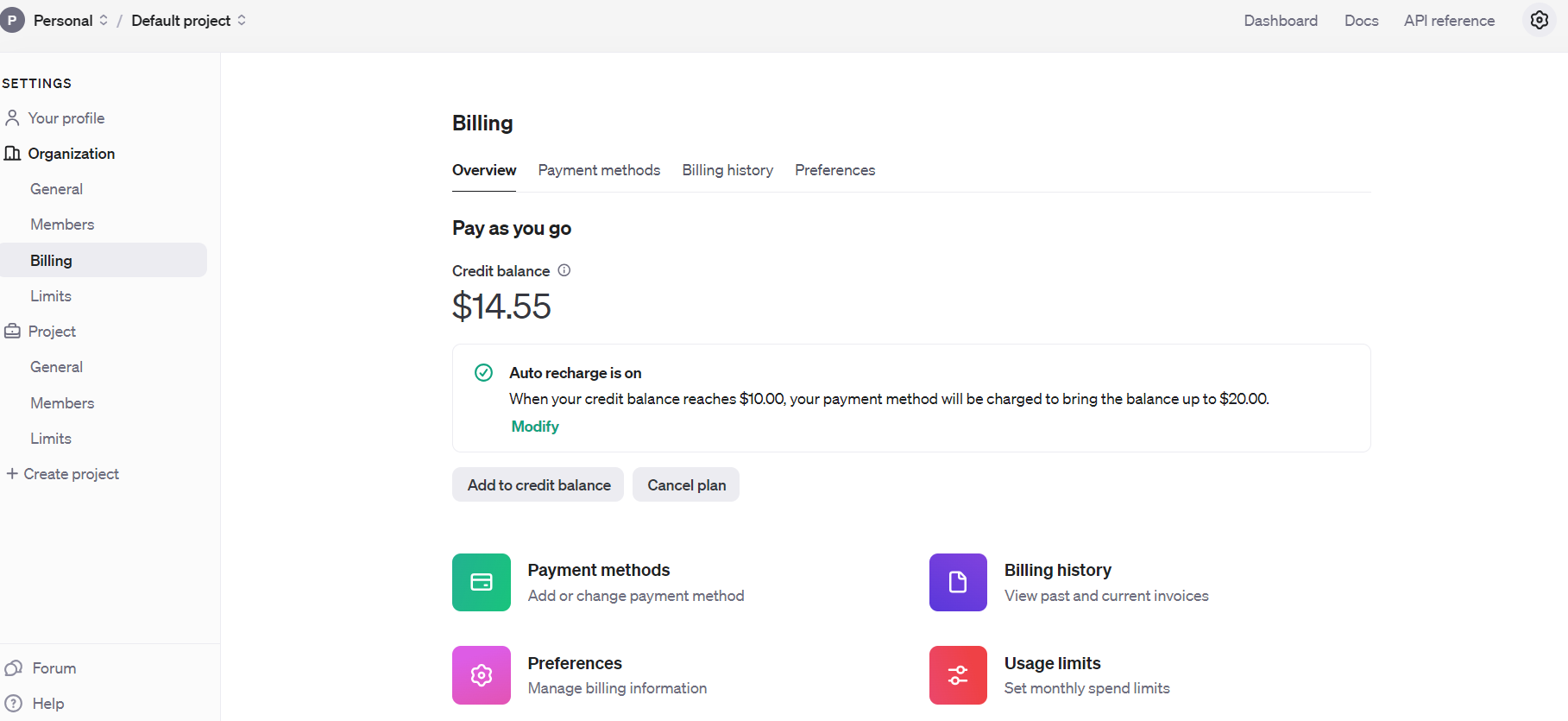 Open AI Api Billing settings
Once you’ve done that, set up email notifications to inform you when your spending exceeds a certain amount under Usage limits.
Then, obtain API keys under Dashboard > API keys, which you should keep private and never share publicly.
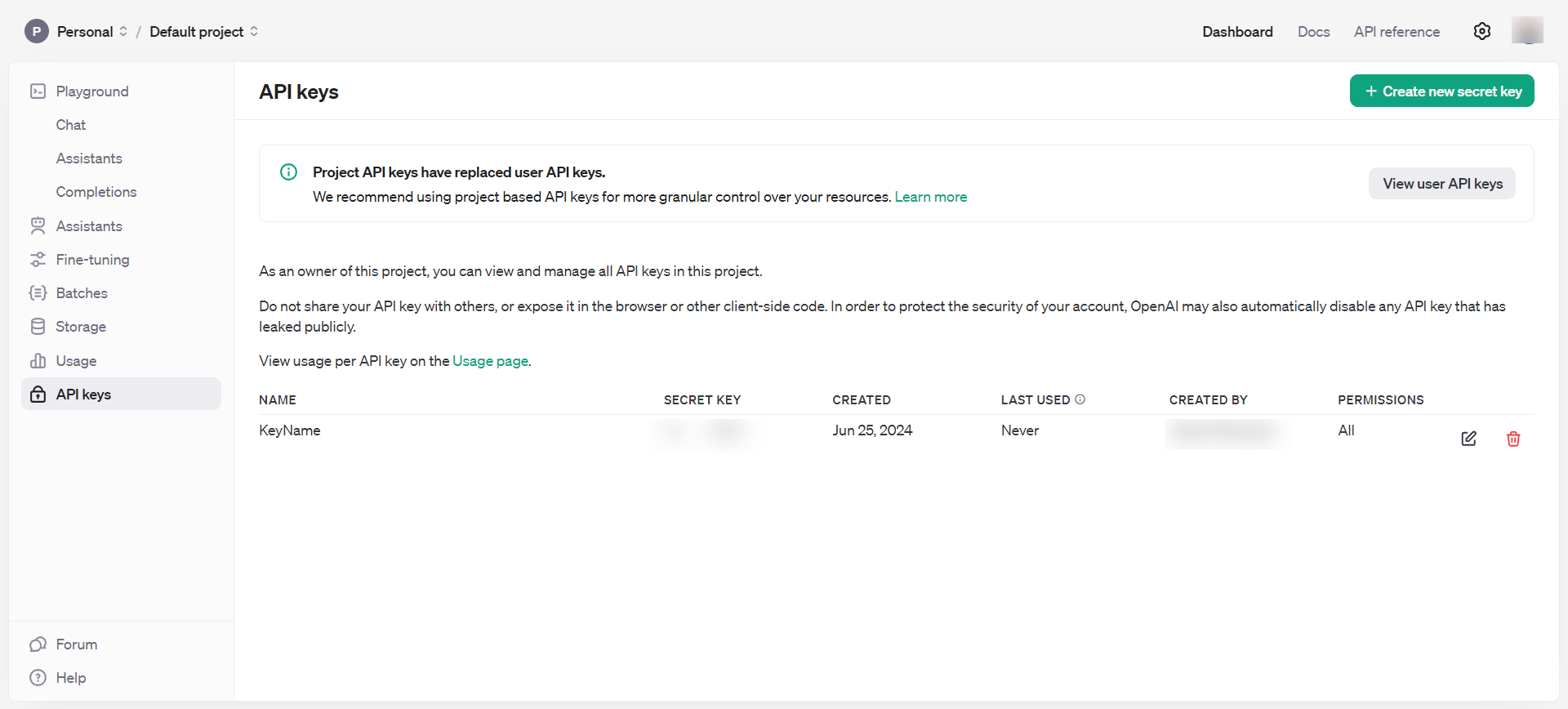 OpenAI API keys
Now, you have all the necessary tools to start playing with embeddings.
- Open your computer command terminal and type
jupyter lab. - You should see something like the below image pop up in your browser.
- Click on Python 3 under Notebook.
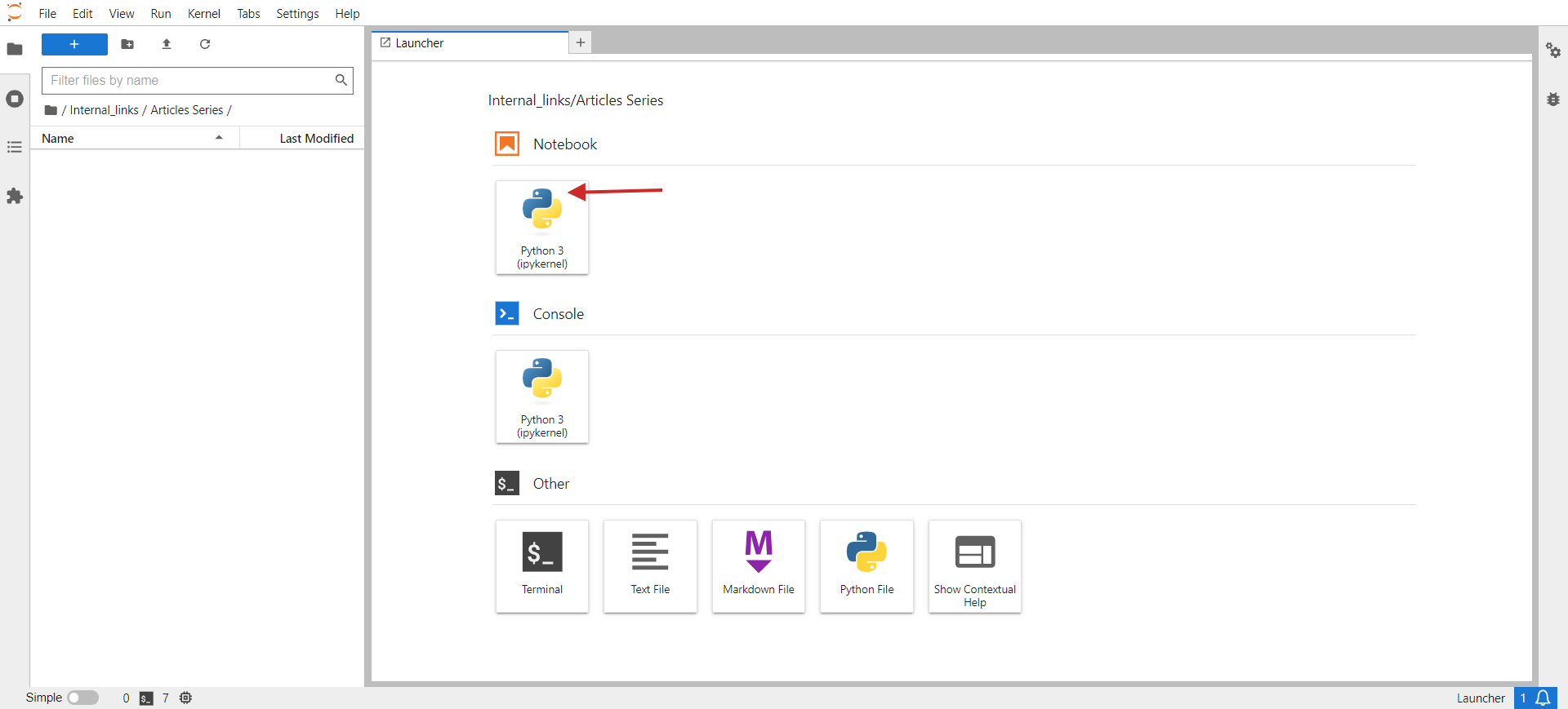 jupyter lab
In the opened window, you will write your code.
As a small task, let’s group similar URLs from a CSV. The sample CSV has two columns: URL and Title. Our script’s task will be to group URLs with similar semantic meanings based on the title so we can consolidate those pages into one and fix keyword cannibalization issues.
Here are the steps you need to do:
Install required Python libraries with the following commands in your PC’s terminal (or in Jupyter notebook)
pip install pandas openai scikit-learn numpy unidecode
The ‘openai’ library is required to interact with the OpenAI API to get embeddings, and ‘pandas’ is used for data manipulation and handling CSV file operations.
The ‘scikit-learn’ library is necessary for calculating cosine similarity, and ‘numpy’ is essential for numerical operations and handling arrays. Lastly, unidecode is used to clean text.
Then, download the sample sheet as a CSV, rename the file to pages.csv, and upload it to your Jupyter folder where your script is located.
Set your OpenAI API key to the key you obtained in the step above, and copy-paste the code below into the notebook.
Run the code by clicking the play triangle icon at the top of the notebook.
import pandas as pd
import openai
from sklearn.metrics.pairwise import cosine_similarity
import numpy as np
import csv
from unidecode import unidecode # Function to clean text
def clean_text(text: str) -> str: # First, replace known problematic characters with their correct equivalents replacements = { '–': '–', # en dash '’': '’', # right single quotation mark '“': '“', # left double quotation mark 'â€': '”', # right double quotation mark '‘': '‘', # left single quotation mark 'â€': '—' # em dash } for old, new in replacements.items(): text = text.replace(old, new) # Then, use unidecode to transliterate any remaining problematic Unicode characters text = unidecode(text) return text # Load the CSV file with UTF-8 encoding from root folder of Jupiter project folder
df = pd.read_csv('pages.csv', encoding='utf-8') # Clean the 'Title' column to remove unwanted symbols
df['Title'] = df['Title'].apply(clean_text) # Set your OpenAI API key
openai.api_key = 'your-api-key-goes-here' # Function to get embeddings
def get_embedding(text): response = openai.Embedding.create(input=[text], engine="text-embedding-ada-002") return response['data'][0]['embedding'] # Generate embeddings for all titles
df['embedding'] = df['Title'].apply(get_embedding) # Create a matrix of embeddings
embedding_matrix = np.vstack(df['embedding'].values) # Compute cosine similarity matrix
similarity_matrix = cosine_similarity(embedding_matrix) # Define similarity threshold
similarity_threshold = 0.9 # since threshold is 0.1 for dissimilarity # Create a list to store groups
groups = [] # Keep track of visited indices
visited = set() # Group similar titles based on the similarity matrix
for i in range(len(similarity_matrix)): if i not in visited: # Find all similar titles similar_indices = np.where(similarity_matrix[i] >= similarity_threshold)[0] # Log comparisons print(f"\nChecking similarity for '{df.iloc[i]['Title']}' (Index {i}):") print("-" * 50) for j in range(len(similarity_matrix)): if i != j: # Ensure that a title is not compared with itself similarity_value = similarity_matrix[i, j] comparison_result = 'greater' if similarity_value >= similarity_threshold else 'less' print(f"Compared with '{df.iloc[j]['Title']}' (Index {j}): similarity = {similarity_value:.4f} ({comparison_result} than threshold)") # Add these indices to visited visited.update(similar_indices) # Add the group to the list group = df.iloc[similar_indices][['URL', 'Title']].to_dict('records') groups.append(group) print(f"\nFormed Group {len(groups)}:") for item in group: print(f" - URL: {item['URL']}, Title: {item['Title']}") # Check if groups were created
if not groups: print("No groups were created.") # Define the output CSV file
output_file = 'grouped_pages.csv' # Write the results to the CSV file with UTF-8 encoding
with open(output_file, 'w', newline='', encoding='utf-8') as csvfile: fieldnames = ['Group', 'URL', 'Title'] writer = csv.DictWriter(csvfile, fieldnames=fieldnames) writer.writeheader() for group_index, group in enumerate(groups, start=1): for page in group: cleaned_title = clean_text(page['Title']) # Ensure no unwanted symbols in the output writer.writerow({'Group': group_index, 'URL': page['URL'], 'Title': cleaned_title}) print(f"Writing Group {group_index}, URL: {page['URL']}, Title: {cleaned_title}") print(f"Output written to {output_file}") This code reads a CSV file, ‘pages.csv,’ containing titles and URLs, which you can easily export from your CMS or get by crawling a client website using Screaming Frog.
Then, it cleans the titles from non-UTF characters, generates embedding vectors for each title using OpenAI’s API, calculates the similarity between the titles, groups similar titles together, and writes the grouped results to a new CSV file, ‘grouped_pages.csv.’
In the keyword cannibalization task, we use a similarity threshold of 0.9, which means if cosine similarity is less than 0.9, we will consider articles as different. To visualize this in a simplified two-dimensional space, it will appear as two vectors with an angle of approximately 25 degrees between them.
<img decoding="async" src="https://marketingnewswired.com/wp-content/uploads/2024/07/find-keyword-cannibalization-using-openais-text-embeddings-with-examples-via-sejournal-vahandev-3.png" alt="
In your case, you may want to use a different threshold, like 0.85 (approximately 31 degrees between them), and run it on a sample of your data to evaluate the results and the overall quality of matches. If it is unsatisfactory, you can increase the threshold to make it more strict for better precision.
You can install ‘matplotlib’ via terminal.
pip install matplotlibAnd use the Python code below in a separate Jupyter notebook to visualize cosine similarities in two-dimensional space on your own. Try it; it’s fun!
import matplotlib.pyplot as plt
import numpy as np # Define the angle for cosine similarity of 0.9. Change here to your desired value. theta = np.arccos(0.9) # Define the vectors
u = np.array([1, 0])
v = np.array([np.cos(theta), np.sin(theta)]) # Define the 45 degree rotation matrix
rotation_matrix = np.array([ [np.cos(np.pi/4), -np.sin(np.pi/4)], [np.sin(np.pi/4), np.cos(np.pi/4)]
]) # Apply the rotation to both vectors
u_rotated = np.dot(rotation_matrix, u)
v_rotated = np.dot(rotation_matrix, v) # Plotting the vectors
plt.figure()
plt.quiver(0, 0, u_rotated[0], u_rotated[1], angles='xy', scale_units='xy', scale=1, color='r')
plt.quiver(0, 0, v_rotated[0], v_rotated[1], angles='xy', scale_units='xy', scale=1, color='b') # Setting the plot limits to only positive ranges
plt.xlim(0, 1.5)
plt.ylim(0, 1.5) # Adding labels and grid
plt.xlabel('X-axis')
plt.ylabel('Y-axis')
plt.grid(True)
plt.title('Visualization of Vectors with Cosine Similarity of 0.9') # Show the plot
plt.show()
I usually use 0.9 and higher for identifying keyword cannibalization issues, but you may need to set it to 0.5 when dealing with old article redirects, as old articles may not have nearly identical articles that are fresher but partially close.
It may also be better to have the meta description concatenated with the title in case of redirects, in addition to the title.
So, it depends on the task you are performing. We will review how to implement redirects in a separate article later in this series.
Now, let’s review the results with the three models mentioned above and see how they were able to identify close articles from our data sample from Search Engine Journal’s articles.
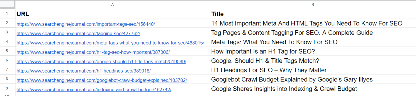 Data Sample
From the list, we already see that the 2nd and 4th articles cover the same topic on ‘meta tags.’ The articles in the 5th and 7th rows are pretty much the same – discussing the importance of H1 tags in SEO – and can be merged.
The article in the 3rd row doesn’t have any similarities with any of the articles in the list but has common words like “Tag” or “SEO.”
The article in the 6th row is again about H1, but not exactly the same as H1’s importance to SEO. Instead, it represents Google’s opinion on whether they should match.
Articles on the 8th and 9th rows are quite close but still different; they can be combined.
text-embedding-ada-002
By using ‘text-embedding-ada-002,’ we precisely found the 2nd and 4th articles with a cosine similarity of 0.92 and the 5th and 7th articles with a similarity of 0.91.
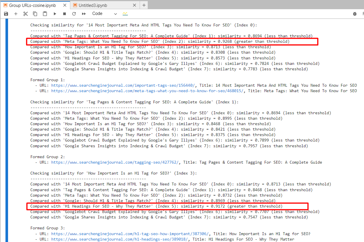 Screenshot from Jupyter log showing cosine similarities
And it generated output with grouped URLs by using the same group number for similar articles. (colors are applied manually for visualization purposes).
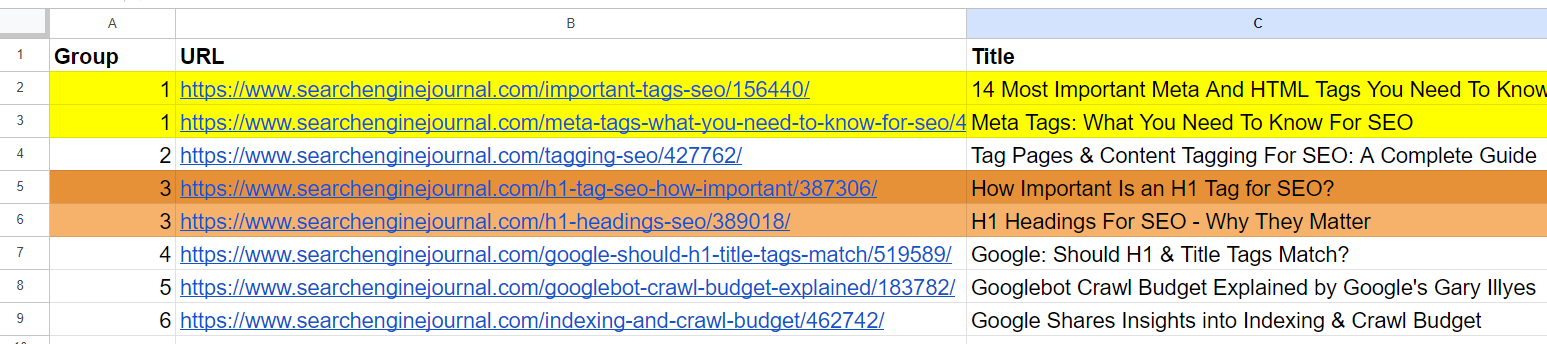 Output sheet with grouped URLs
For the 2nd and 3rd articles, which have common words “Tag” and “SEO” but are unrelated, the cosine similarity was 0.86. This shows why a high similarity threshold of 0.9 or greater is necessary. If we set it to 0.85, it would be full of false positives and could suggest merging unrelated articles.
text-embedding-3-small
By using ‘text-embedding-3-small,’ quite surprisingly, it didn’t find any matches per our similarity threshold of 0.9 or higher.
For the 2nd and 4th articles, cosine similarity was 0.76, and for the 5th and 7th articles, with similarity 0.77.
To better understand this model through experimentation, I’ve added a slightly modified version of the 1st row with ’15’ vs. ’14’ to the sample.
- “14 Most Important Meta And HTML Tags You Need To Know For SEO”
- “15 Most Important Meta And HTML Tags You Need To Know For SEO”
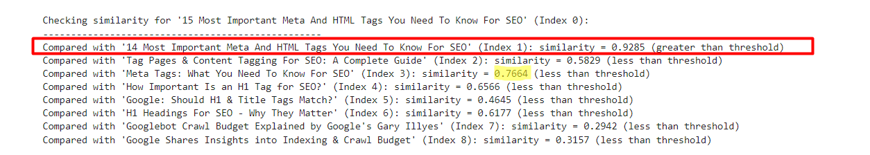 An example which shows text-embedding-3-small results
On the contrary, ‘text-embedding-ada-002’ gave 0.98 cosine similarity between those versions.
| Title 1 | Title 2 | Cosine Similarity |
| 14 Most Important Meta And HTML Tags You Need To Know For SEO | 15 Most Important Meta And HTML Tags You Need To Know For SEO | 0.92 |
| 14 Most Important Meta And HTML Tags You Need To Know For SEO | Meta Tags: What You Need To Know For SEO | 0.76 |
Here, we see that this model is not quite a good fit for comparing titles.
text-embedding-3-large
This model’s dimensionality is 3072, which is 2 times higher than that of ‘text-embedding-3-small’ and ‘text-embedding-ada-002′, with 1536 dimensionality.
As it has more dimensions than the other models, we could expect it to capture semantic meaning with higher precision.
However, it gave the 2nd and 4th articles cosine similarity of 0.70 and the 5th and 7th articles similarity of 0.75.
I’ve tested it again with slightly modified versions of the first article with ’15’ vs. ’14’ and without ‘Most Important’ in the title.
- “14 Most Important Meta And HTML Tags You Need To Know For SEO”
- “15 Most Important Meta And HTML Tags You Need To Know For SEO”
- “14 Meta And HTML Tags You Need To Know For SEO”
| Title 1 | Title 2 | Cosine Similarity |
| 14 Most Important Meta And HTML Tags You Need To Know For SEO | 15 Most Important Meta And HTML Tags You Need To Know For SEO | 0.95 |
| 14 Most Important Meta And HTML Tags You Need To Know For SEO | 14 |
0.93 |
| 14 Most Important Meta And HTML Tags You Need To Know For SEO | Meta Tags: What You Need To Know For SEO | 0.70 |
| 15 Most Important Meta And HTML Tags You Need To Know For SEO | 14 |
0.86 |
So we can see that ‘text-embedding-3-large’ is underperforming compared to ‘text-embedding-ada-002’ when we calculate cosine similarities between titles.
I want to note that the accuracy of ‘text-embedding-3-large’ increases with the length of the text, but ‘text-embedding-ada-002’ still performs better overall.
Another approach could be to strip away stop words from the text. Removing these can sometimes help focus the embeddings on more meaningful words, potentially improving the accuracy of tasks like similarity calculations.
The best way to determine whether removing stop words improves accuracy for your specific task and dataset is to empirically test both approaches and compare the results.
Conclusion
With these examples, you have learned how to work with OpenAI’s embedding models and can already perform a wide range of tasks.
For similarity thresholds, you need to experiment with your own datasets and see which thresholds make sense for your specific task by running it on smaller samples of data and performing a human review of the output.
Please note that the code we have in this article is not optimal for large datasets since you need to create text embeddings of articles every time there is a change in your dataset to evaluate against other rows.
To make it efficient, we must use vector databases and store embedding information there once generated. We will cover how to use vector databases very soon and change the code sample here to use a vector database.
More resources:
Featured Image: BestForBest/Shutterstock