Transitioning From Excel To Python: Essential Functions For SEO Data Analysis via @sejournal, @williamjnye

Learning to code, whether with Python, JavaScript, or another programming language, has a whole host of benefits, including the ability to work with larger datasets and automate repetitive tasks.

But despite the benefits, many SEO professionals are yet to make the transition – and I completely understand why! It isn’t an essential skill for SEO, and we’re all busy people.

If you’re pressed for time, and you already know how to accomplish a task within Excel or Google Sheets, then changing tack can feel like reinventing the wheel.

When I first started coding, I initially only used Python for tasks that I couldn’t accomplish in Excel – and it’s taken several years to get to the point where it’s my defacto choice for data processing.

Looking back, I’m incredibly glad that I persisted, but at times it was a frustrating experience, with many an hour spent scanning threads on Stack Overflow.

This post is designed to spare other SEO pros the same fate.

Within it, we’ll cover the Python equivalents of the most commonly used Excel formulas and features for SEO data analysis – all of which are available within a Google Colab notebook linked in the summary.

Specifically, you’ll learn the equivalents of:

• LEN.
• Drop Duplicates.
• Text to Columns.
• SEARCH/FIND.
• CONCATENATE.
• Find and Replace.
• LEFT/MID/RIGHT.
• IF.
• IFS.
• VLOOKUP.
• COUNTIF/SUMIF/AVERAGEIF.
• Pivot Tables.

Amazingly, to accomplish all of this, we’ll primarily be using a singular library – Pandas – with a little help in places from its big brother, NumPy.

Prerequisites

For the sake of brevity, there are a few things we won’t be covering today, including:

• Installing Python.
• Basic Pandas, like importing CSVs, filtering, and previewing dataframes.

If you’re unsure about any of this, then Hamlet’s guide on Python data analysis for SEO is the perfect primer.

Now, without further ado, let’s jump in.

LEN

LEN provides a count of the number of characters within a string of text.

For SEO specifically, a common use case is to measure the length of title tags or meta descriptions to determine whether they’ll be truncated in search results.

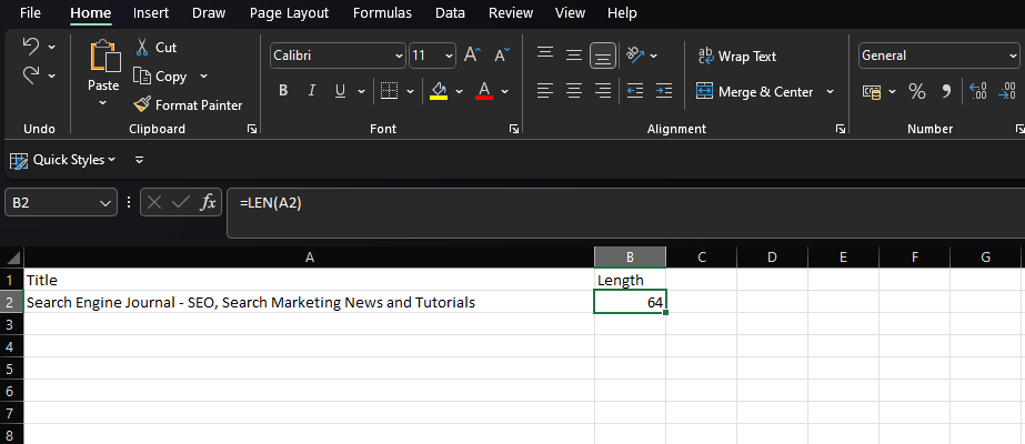
Within Excel, if we wanted to count the second cell of column A, we’d enter:

=LEN(A2)

Python isn’t too dissimilar, as we can rely on the inbuilt len function, which can be combined with Pandas’ loc[] to access a specific row of data within a column:

len(df['Title'].loc[0])

In this example, we’re getting the length of the first row in the “Title” column of our dataframe.

Finding the length of a cell isn’t that useful for SEO, though. Normally, we’d want to apply a function to an entire column!

In Excel, this would be achieved by selecting the formula cell on the bottom right-hand corner and either dragging it down or double-clicking.

When working with a Pandas dataframe, we can use str.len to calculate the length of rows within a series, then store the results in a new column:

df['Length'] = df['Title'].str.len()

Str.len is a ‘vectorized’ operation, which is designed to be applied simultaneously to a series of values. We’ll use these operations extensively throughout this article, as they almost universally end up being faster than a loop.

Another common application of LEN is to combine it with SUBSTITUTE to count the number of words in a cell:

=LEN(TRIM(A2))-LEN(SUBSTITUTE(A2," ",""))+1

In Pandas, we can achieve this by combining the str.split and str.len functions together:

df['No. Words'] = df['Title'].str.split().str.len()

We’ll cover str.split in more detail later, but essentially, what we’re doing is splitting our data based upon whitespaces within the string, then counting the number of component parts.

Dropping Duplicates

Excel’s ‘Remove Duplicates’ feature provides an easy way to remove duplicate values within a dataset, either by deleting entirely duplicate rows (when all columns are selected) or removing rows with the same values in specific columns.

In Pandas, this functionality is provided by drop_duplicates.

To drop duplicate rows within a dataframe type:

df.drop_duplicates(inplace=True)

To drop rows based on duplicates within a singular column, include the subset parameter:

df.drop_duplicates(subset='column', inplace=True)

Or specify multiple columns within a list:

df.drop_duplicates(subset=['column','column2'], inplace=True)

One addition above that’s worth calling out is the presence of the inplace parameter. Including inplace=True allows us to overwrite our existing dataframe without needing to create a new one.

There are, of course, times when we want to preserve our raw data. In this case, we can assign our deduped dataframe to a different variable:

df2 = df.drop_duplicates(subset='column')

Text To Columns

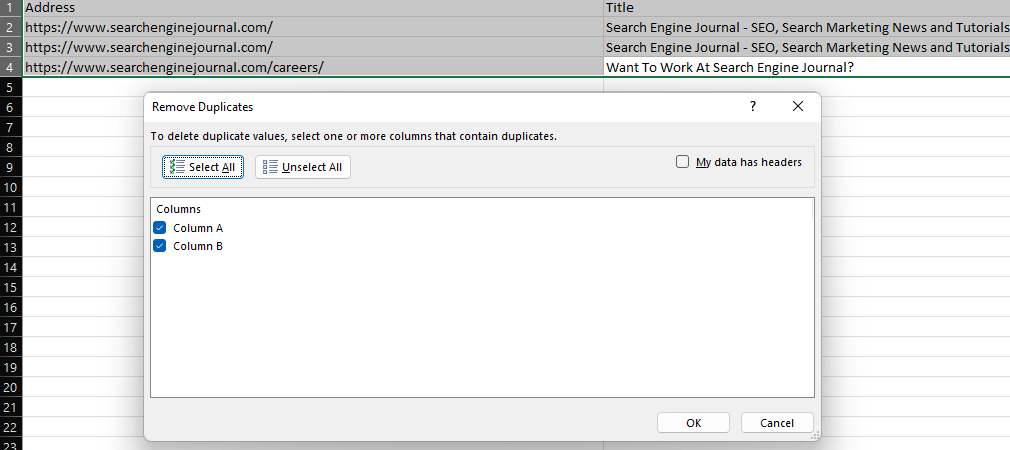
Another everyday essential, the ‘text to columns’ feature can be used to split a text string based on a delimiter, such as a slash, comma, or whitespace.

As an example, splitting a URL into its domain and individual subfolders.

When dealing with a dataframe, we can use the str.split function, which creates a list for each entry within a series. This can be converted into multiple columns by setting the expand parameter to True:

df['URL'].str.split(pat='/', expand=True)

As is often the case, our URLs in the image above have been broken up into inconsistent columns, because they don’t feature the same number of folders.

This can make things tricky when we want to save our data within an existing dataframe.

Specifying the n parameter limits the number of splits, allowing us to create a specific number of columns:

df[['Domain', 'Folder1', 'Folder2', 'Folder3']] = df['URL'].str.split(pat='/', expand=True, n=3)

Another option is to use pop to remove your column from the dataframe, perform the split, and then re-add it with the join function:

df = df.join(df.pop('Split').str.split(pat='/', expand=True))

Duplicating the URL to a new column before the split allows us to preserve the full URL. We can then rename the new columns:🐆

df['Split'] = df['URL'] df = df.join(df.pop('Split').str.split(pat='/', expand=True)) df.rename(columns = {0:'Domain', 1:'Folder1', 2:'Folder2', 3:'Folder3', 4:'Parameter'}, inplace=True)

CONCATENATE

The CONCAT function allows users to combine multiple strings of text, such as when generating a list of keywords by adding different modifiers.

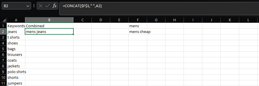
In this case, we’re adding “mens” and whitespace to column A’s list of product types:

=CONCAT($F$1," ",A2)

Assuming we’re dealing with strings, the same can be achieved in Python using the arithmetic operator:

df['Combined] = 'mens' + ' ' + df['Keyword']

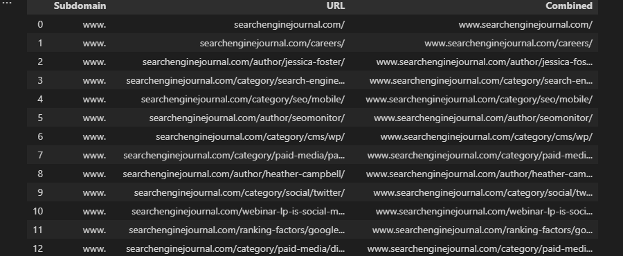
Or specify multiple columns of data:

df['Combined'] = df['Subdomain'] + df['URL']

Pandas has a dedicated concat function, but this is more useful when trying to combine multiple dataframes with the same columns.

For instance, if we had multiple exports from our favorite link analysis tool:

df = pd.read_csv('data.csv')
df2 = pd.read_csv('data2.csv')
df3 = pd.read_csv('data3.csv') dflist = [df, df2, df3] df = pd.concat(dflist, ignore_index=True)

SEARCH/FIND

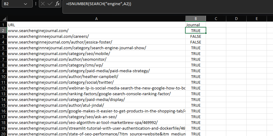
The SEARCH and FIND formulas provide a way of locating a substring within a text string.

These commands are commonly combined with ISNUMBER to create a Boolean column that helps filter down a dataset, which can be extremely helpful when performing tasks like log file analysis, as explained in this guide. E.g.:

=ISNUMBER(SEARCH("searchthis",A2)

The difference between SEARCH and FIND is that find is case-sensitive.

The equivalent Pandas function, str.contains, is case-sensitive by default:

df['Journal'] = df['URL'].str.contains('engine', na=False)

Case insensitivity can be enabled by setting the case parameter to False:

df['Journal'] = df['URL'].str.contains('engine', case=False, na=False)

In either scenario, including na=False will prevent null values from being returned within the Boolean column.

One massive advantage of using Pandas here is that, unlike Excel, regex is natively supported by this function – as it is in Google sheets via REGEXMATCH.

Chain together multiple substrings by using the pipe character, also known as the OR operator:

df['Journal'] = df['URL'].str.contains('engine|search', na=False)

Find And Replace

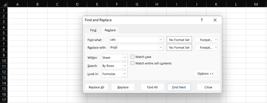
Excel’s “Find and Replace” feature provides an easy way to individually or bulk replace one substring with another.

When processing data for SEO, we’re most likely to select an entire column and “Replace All.”

The SUBSTITUTE formula provides another option here and is useful if you don’t want to overwrite the existing column.

As an example, we can change the protocol of a URL from HTTP to HTTPS, or remove it by replacing it with nothing.

When working with dataframes in Python, we can use str.replace:

df['URL'] = df['URL'].str.replace('http://', 'https://')

Or:

df['URL'] = df['URL'].str.replace('http://', '') # replace with nothing

Again, unlike Excel, regex can be used – like with Google Sheets’ REGEXREPLACE:

df['URL'] = df['URL'].str.replace('http://|https://', '')

Alternatively, if you want to replace multiple substrings with different values, you can use Python’s replace method and provide a list.

This prevents you from having to chain multiple str.replace functions:

df['URL'] = df['URL'].replace(['http://', ' https://'], ['https://www.', 'https://www.’], regex=True)

LEFT/MID/RIGHT

Extracting a substring within Excel requires the usage of the LEFT, MID, or RIGHT functions, depending on where the substring is located within a cell.

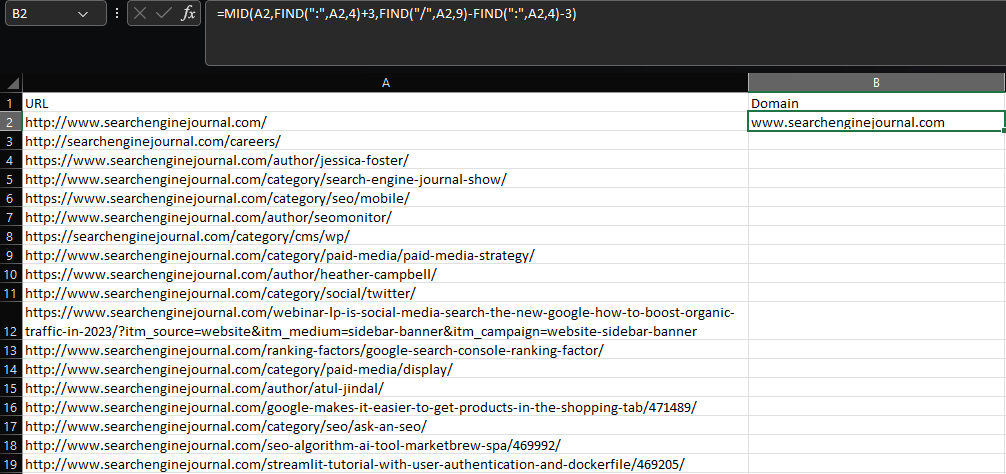
Let’s say we want to extract the root domain and subdomain from a URL:

=MID(A2,FIND(":",A2,4)+3,FIND("/",A2,9)-FIND(":",A2,4)-3)

Using a combination of MID and multiple FIND functions, this formula is ugly, to say the least – and things get a lot worse for more complex extractions.

Again, Google Sheets does this better than Excel, because it has REGEXEXTRACT.

What a shame that when you feed it larger datasets, it melts faster than a Babybel on a hot radiator.

Thankfully, Pandas offers str.extract, which works in a similar way:

df['Domain'] = df['URL'].str.extract('.*\://?([^\/]+)')

Combine with fillna to prevent null values, as you would in Excel with IFERROR:

df['Domain'] = df['URL'].str.extract('.*\://?([^\/]+)').fillna('-')

If

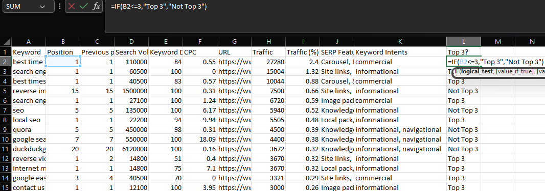
IF statements allow you to return different values, depending on whether or not a condition is met.

To illustrate, suppose that we want to create a label for keywords that are ranking within the top three positions.

Rather than using Pandas in this instance, we can lean on NumPy and the where function (remember to import NumPy, if you haven’t already):

df['Top 3'] = np.where(df['Position'] <= 3, 'Top 3', 'Not Top 3')

Multiple conditions can be used for the same evaluation by using the AND/OR operators, and enclosing the individual criteria within round brackets:

df['Top 3'] = np.where((df['Position'] <= 3) & (df['Position'] != 0), 'Top 3', 'Not Top 3')

In the above, we’re returning “Top 3” for any keywords with a ranking less than or equal to three, excluding any keywords ranking in position zero.

IFS

Sometimes, rather than specifying multiple conditions for the same evaluation, you may want multiple conditions that return different values.

In this case, the best solution is using IFS:

=IFS(B2<=3,"Top 3",B2<=10,"Top 10",B2<=20,"Top 20")

Again, NumPy provides us with the best solution when working with dataframes, via its select function.

With select, we can create a list of conditions, choices, and an optional value for when all of the conditions are false:

conditions = [df['Position'] <= 3, df['Position'] <= 10, df['Position'] <=20] choices = ['Top 3', 'Top 10', 'Top 20'] df['Rank'] = np.select(conditions, choices, 'Not Top 20')

It’s also possible to have multiple conditions for each of the evaluations.

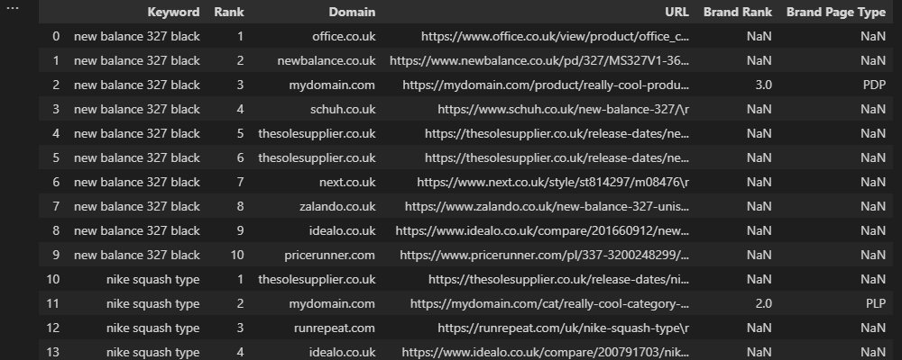
Let’s say we’re working with an ecommerce retailer with product listing pages (PLPs) and product display pages (PDPs), and we want to label the type of branded pages ranking within the top 10 results.

The easiest solution here is to look for specific URL patterns, such as a subfolder or extension, but what if competitors have similar patterns?

In this scenario, we could do something like this:

conditions = [(df['URL'].str.contains('/category/')) & (df['Brand Rank'] > 0),
(df['URL'].str.contains('/product/')) & (df['Brand Rank'] > 0),
(~df['URL'].str.contains('/product/')) & (~df['URL'].str.contains('/category/')) & (df['Brand Rank'] > 0)] choices = ['PLP', 'PDP', 'Other'] df['Brand Page Type'] = np.select(conditions, choices, None)

Above, we’re using str.contains to evaluate whether or not a URL in the top 10 matches our brand’s pattern, then using the “Brand Rank” column to exclude any competitors.

In this example, the tilde sign (~) indicates a negative match. In other words, we’re saying we want every brand URL that doesn’t match the pattern for a “PDP” or “PLP” to match the criteria for ‘Other.’

Lastly, None is included because we want non-brand results to return a null value.

VLOOKUP

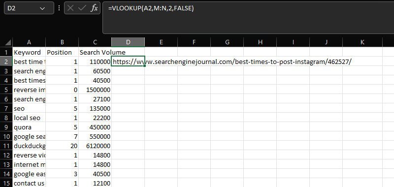
VLOOKUP is an essential tool for joining together two distinct datasets on a common column.

In this case, adding the URLs within column N to the keyword, position, and search volume data in columns A-C, using the shared “Keyword” column:

=VLOOKUP(A2,M:N,2,FALSE)

To do something similar with Pandas, we can use merge.

Replicating the functionality of an SQL join, merge is an incredibly powerful function that supports a variety of different join types.

For our purposes, we want to use a left join, which will maintain our first dataframe and only merge in matching values from our second dataframe:

mergeddf = df.merge(df2, how='left', on='Keyword')

One added advantage of performing a merge over a VLOOKUP, is that you don’t have to have the shared data in the first column of the second dataset, as with the newer XLOOKUP.

It will also pull in multiple rows of data rather than the first match in finds.

One common issue when using the function is for unwanted columns to be duplicated. This occurs when multiple shared columns exist, but you attempt to match using one.

To prevent this – and improve the accuracy of your matches – you can specify a list of columns:

mergeddf = df.merge(df2, how='left', on=['Keyword', 'Search Volume'])

In certain scenarios, you may actively want these columns to be included. For instance, when attempting to merge multiple monthly ranking reports:

mergeddf = df.merge(df2, on='Keyword', how='left', suffixes=('', '_october'))\ .merge(df3, on='Keyword', how='left', suffixes=('', '_september'))

The above code snippet executes two merges to join together three dataframes with the same columns – which are our rankings for November, October, and September.

By labeling the months within the suffix parameters, we end up with a much cleaner dataframe that clearly displays the month, as opposed to the defaults of _x and _y seen in the earlier example.

COUNTIF/SUMIF/AVERAGEIF

In Excel, if you want to perform a statistical function based on a condition, you’re likely to use either COUNTIF, SUMIF, or AVERAGEIF.

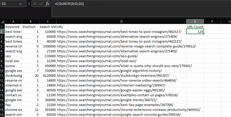
Commonly, COUNTIF is used to determine how many times a specific string appears within a dataset, such as a URL.

We can accomplish this by declaring the ‘URL’ column as our range, then the URL within an individual cell as our criteria:

=COUNTIF(D:D,D2)

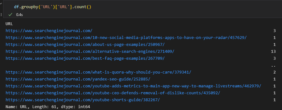
In Pandas, we can achieve the same outcome by using the groupby function:

df.groupby('URL')['URL'].count()

Here, the column declared within the round brackets indicates the individual groups, and the column listed in the square brackets is where the aggregation (i.e., the count) is performed.

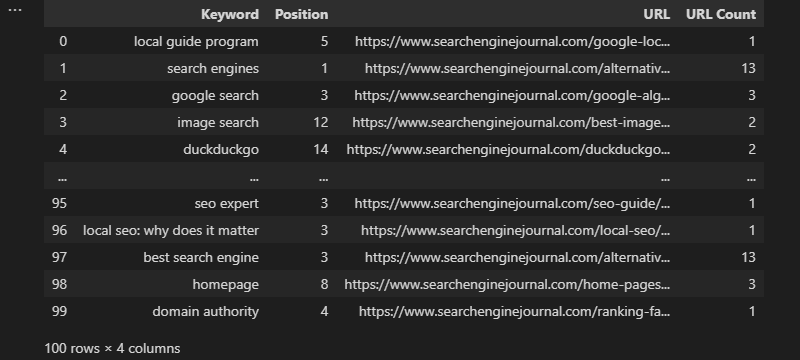
The output we’re receiving isn’t perfect for this use case, though, because it’s consolidated the data.

Typically, when using Excel, we’d have the URL count inline within our dataset. Then we can use it to filter to the most frequently listed URLs.

To do this, use transform and store the output in a column:

df['URL Count'] = df.groupby('URL')['URL'].transform('count')

You can also apply custom functions to groups of data by using a lambda (anonymous) function:

df['Google Count'] = df.groupby(['URL'])['URL'].transform(lambda x: x[x.str.contains('google')].count())

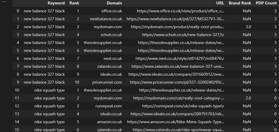
In our examples so far, we’ve been using the same column for our grouping and aggregations, but we don’t have to. Similarly to COUNTIFS/SUMIFS/AVERAGEIFS in Excel, it’s possible to group using one column, then apply our statistical function to another.

Going back to the earlier search engine results page (SERP) example, we may want to count all ranking PDPs on a per-keyword basis and return this number alongside our existing data:

df['PDP Count'] = df.groupby(['Keyword'])['URL'].transform(lambda x: x[x.str.contains('/product/|/prd/|/pd/')].count())

=SUM(COUNTIFS(A:A,[@Keyword],D:D,{"*/product/*","*/prd/*","*/pd/*"}))

Pivot Tables

Last, but by no means least, it’s time to talk pivot tables.

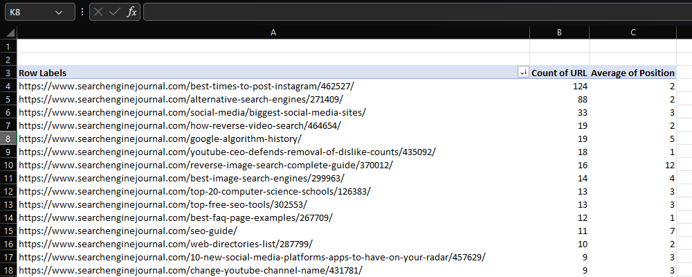
In Excel, a pivot table is likely to be our first port of call if we want to summarise a large dataset.

For instance, when working with ranking data, we may want to identify which URLs appear most frequently, and their average ranking position.

Again, Pandas has its own pivot tables equivalent – but if all you want is a count of unique values within a column, this can be accomplished using the value_counts function:

count = df['URL'].value_counts()

Using groupby is also an option.

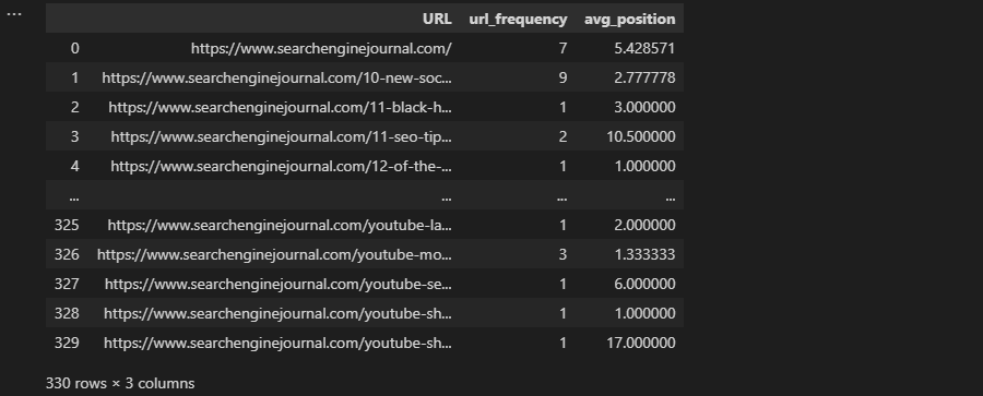
Earlier in the article, performing a groupby that aggregated our data wasn’t what we wanted – but it’s precisely what’s required here:

grouped = df.groupby('URL').agg( url_frequency=('Keyword', 'count'), avg_position=('Position', 'mean'), ) grouped.reset_index(inplace=True)

Two aggregate functions have been applied in the example above, but this could easily be expanded upon, and 13 different types are available.

There are, of course, times when we do want to use pivot_table, such as when performing multi-dimensional operations.

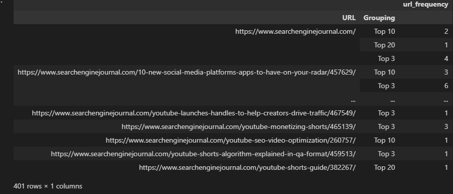
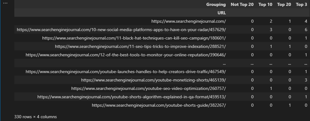
To illustrate what this means, let’s reuse the ranking groupings we made using conditional statements and attempt to display the number of times a URL ranks within each group.

ranking_groupings = df.groupby(['URL', 'Grouping']).agg( url_frequency=('Keyword', 'count'), )

This isn’t the best format to use, as multiple rows have been created for each URL.

Instead, we can use pivot_table, which will display the data in different columns:

pivot = pd.pivot_table(df,
index=['URL'],
columns=['Grouping'],
aggfunc='size',
fill_value=0,
)

Final Thoughts

Whether you’re looking for inspiration to start learning Python, or are already leveraging it in your SEO workflows, I hope that the above examples help you along on your journey.

As promised, you can find a Google Colab notebook with all of the code snippets here.

In truth, we’ve barely scratched the surface of what’s possible, but understanding the basics of Python data analysis will give you a solid base upon which to build.

More resources:

---

Featured Image: mapo_japan/Shutterstock